Wireless Power Transfer
Fast Simulation
AirInduct Sim is a physics-backed electromagnetic simulation platform for WPT coil research. Model magnetic field coupling, mutual inductance, and energy transfer across 8 validated coil topologies — on web and mobile.

Built on real physics. Engineered for research.
Four outputs. Three render modes. Three platforms. One Biot–Savart kernel, running on eight validated topologies — covered end to end by the same frozen benchmark suite.
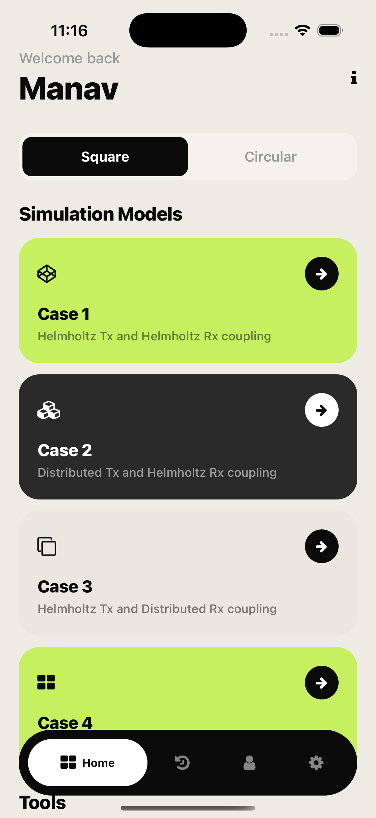
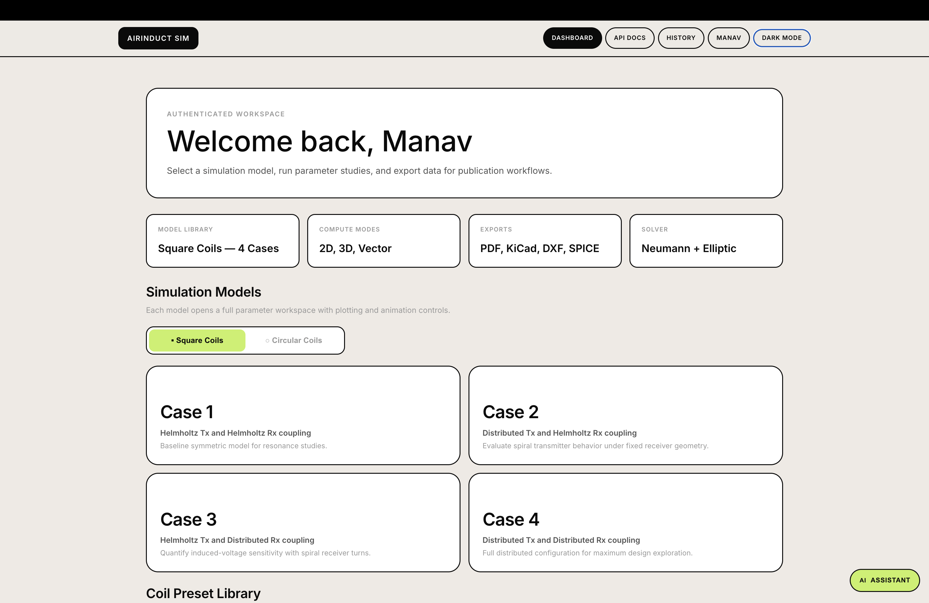
Four square and four circular coils — Helmholtz, DTC-Helm, Helm-DTC, DTC-DTC — each with its own validated solver.
2d_plane heatmaps, 3d_volume isosurfaces, vector_field arrows. One tensor, three views.
M, L_tx, L_rx, Vout, Hx_max, Hy_max, Hz_max — from Biot–Savart plus Neumann, no surrogates.
Web dashboard, native iOS/Android, and a REST API in development — all running the same solver.
The only WPT platform that takes you from coil geometry to coupling factor to CAD export in one session.
See the Invisible
Full 3D volumetric magnetic field maps — Hx, Hy, Hz components plus |B| magnitude. Up to 500 × 500 resolution grid computed via vectorized Biot-Savart law.
8 Coil Topologies
4 square + 4 circular geometries. Helmholtz ↔ Distributed in every Tx/Rx combo.
Dial In Every Variable
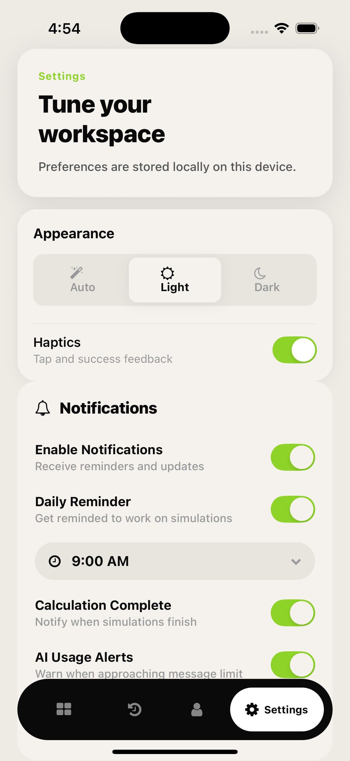
13 tunable parameters per simulation. Sliders update the field in real time.
2D for Speed. 3D for Depth.
Three render modes from every simulation.
Numbers That Matter
First-principles output you can cite.
Optimize Automatically
Genetic algorithm + parameter sweep. Set a target k, sweep 2–100 steps across any variable, get Pareto-optimal geometries.
Export Everything
One-click exports from every run.
From Simulation to Hardware
Every result maps to exact input parameters. Export coupling data, field maps, and coil geometry to your PCB layout, CAD tool, or publication.
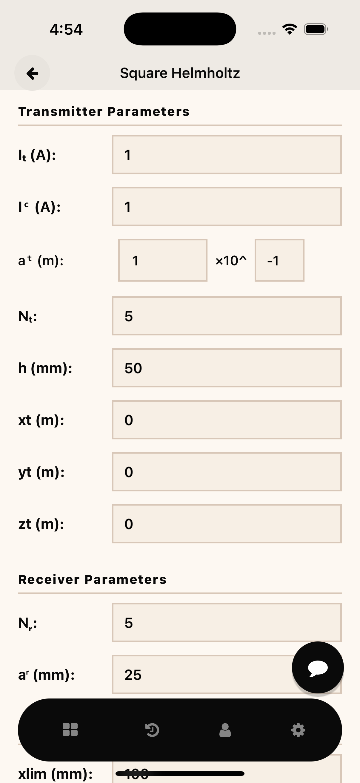
13 tunable parameters per simulation — current (I, Ic), frequency, coil dimensions (amax, R), turn count (Nr, Nt), position (xt, yt, zt), spacing, and resolution. Results update in seconds.

Not Another Slow FEM Tool.
Real Physics. Real Speed.
Vectorized Biot-Savart computation delivers full 3D electromagnetic field maps in seconds — not hours. No mesh generation. No convergence issues. No FEM license fees.
Sweep Any Parameter Instantly
Animate height, current, or coil radius across 2–100 steps in a single sweep. Watch coupling factor evolve from k = 0.01 to k = 0.30 as you vary spacing from 20 mm to 100 mm. No manual re-runs.
First-Principles Output You Can Cite
Every simulation returns: mutual inductance (M), self-inductance (L_tx, L_rx), induced voltage (Vout), and peak field components (Hx_max, Hy_max, Hz_max) — all from Biot-Savart + Neumann formula. Coupling k is derived as M/√(L_tx · L_rx). No curve fitting. No surrogate models.
Built for Integration. API Coming Soon.
Every topology runs on a validated Biot-Savart solver — Helmholtz, DTC-Helmholtz, Helmholtz-DTC, DTC-DTC in both square and circular geometries. A full REST API with 22 endpoints is in development for pipeline and CI integration.
Our solvers are tested against real IEEE papers and textbook solutions. If a number doesn't match the reference within tolerance, we don't ship it.
Case 1 Helmholtz, default parameters. These are real solver inputs and outputs — not mockups.
WPT Research Papers
Sweep spacing from 10mm to 200mm, plot k vs. separation, cite the Babic 2008 reference values in your paper.
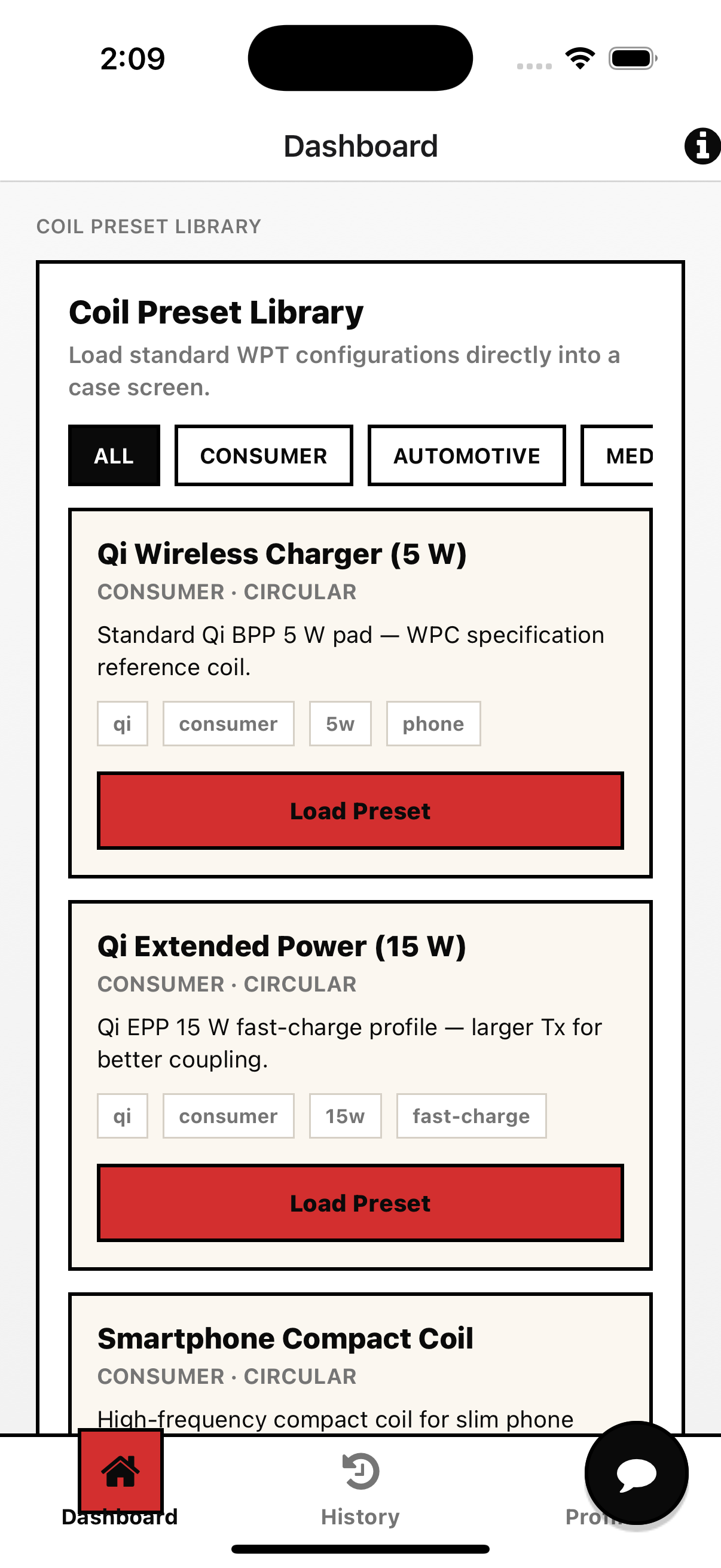
Coil Prototyping
Simulate, optimize with the genetic algorithm, then export a .kicad_mod footprint and DXF outline.
EV Charging
SAE J2954 at 85 kHz. LCC-LCC matching. η > 90%.
Medical Implants
Miniature Rx (R < 10mm). Verify Hz_max safety limits.
IoT Sensors
Compact coils, max k at small form factors. SPICE out.
Teaching Labs
Interactive sliders, real-time heatmaps, PDF lab reports.
Your Coil Design Deserves
Better Tools Than a Spreadsheet.
Pick a topology. Set your parameters. Get field maps, coupling factor k, and inductance values in seconds. Export to PDF, KiCad, DXF, or SPICE. Ship your design.
Start Simulating